Train YOLOv8 on a Custom Dataset in Google Colab

Pretrained YOLO models know 80 everyday objects: people, cars, dogs, cups. Real projects almost always need something else: number plates, helmets, potholes, cracks in concrete. The fastest way to get there is to fine-tune a pretrained YOLOv8 model on your own labelled images.

This guide walks through the full process in Google Colab, from an empty notebook to a trained model you can run on images and video. As a running example I use my own car number plate detector: a labelled dataset from Roboflow, a free Colab T4 GPU and the Ultralytics YOLOv8 package. The final model reached 97.9% mAP@50 and 99.1% precision on its validation set, although, as you'll see below, it took me three training runs to get there.

What you need

• A Google account for Google Colab. The free tier is enough to start.
• Images of the object you want to detect, with bounding-box labels in YOLO format. I used a number plate dataset from Roboflow Universe, which exports straight to YOLOv8 format. CVAT and Label Studio work too if you label your own images.
• Time. A small dataset trains in under an hour; my final 50-epoch run took about 3.2 hours on a T4.

Step 1: Switch Colab to a GPU

Training on a CPU is painfully slow. In Colab, open Runtime → Change runtime type and pick a GPU, then check that it's there:

!nvidia-smi

You should see a table with the GPU name and memory. On the free tier I got an NVIDIA T4, which is plenty for a nano or small YOLO model. If you get an error, the runtime is still on CPU.

Step 2: Install Ultralytics

YOLOv8 is published by Ultralytics as a Python package:

!pip install ultralytics

import ultralytics
ultralytics.checks()

checks() prints the installed version, Python, PyTorch and whether CUDA (the GPU) is available.

Step 3: Prepare the dataset

YOLO expects one image folder and one label folder per split. Each image has a .txt file with the same name in the matching labels folder:

dataset/
├── data.yaml
├── train/
│   ├── images/   car_001.jpg, car_002.jpg, ...
│   └── labels/   car_001.txt, car_002.txt, ...
└── valid/
    ├── images/
    └── labels/

Each line in a label file describes one object:

0 0.512 0.634 0.180 0.062

The five numbers are the class index, then the box centre (x, y), width and height. All four box values are normalised to 0–1 by the image width and height, not in pixels. An image with no objects can have an empty label file; YOLO treats it as a background example, which helps reduce false positives.

The data.yaml file

data.yaml tells YOLO where the splits are and what each class index means. For a single-class detector like mine:

path: /content/dataset
train: train/images
val: valid/images

names:
  0: number_plate

For more classes, keep adding lines (1: helmet, 2: no_helmet, and so on). The indices must match the first number in your label files.

Getting the data into Colab

If your data is on Roboflow, open the dataset version, click Export, choose the YOLOv8 format and download the zip. It already has the folder layout above and a data.yaml.

The simplest way to get the zip into Colab is through Google Drive: upload it there, then unzip it onto the Colab machine. Reading thousands of small files directly from Drive is slow, so copy it to local disk first:

from google.colab import drive
drive.mount('/content/drive')

!unzip -q /content/drive/MyDrive/dataset.zip -d /content/

Check that /content/dataset/data.yaml exists before moving on, and open it once: exported files sometimes contain relative paths like ../train/images that don't match where you unzipped. A wrong path here causes the most common error at the next step: dataset not found.

Step 4: Train the model

Start from pretrained weights rather than from scratch. The model already understands edges, shapes and textures, so it only has to learn your object:

from ultralytics import YOLO

model = YOLO("yolov8n.pt")  # nano: smallest and fastest

results = model.train(
    data="/content/dataset/data.yaml",
    epochs=50,
    imgsz=640,
    batch=16,
)

These are exactly the settings I used for the number plate model. What each one means:

Setting	Value	Why
yolov8n.pt	nano model, about 3M parameters	Fast and small (my trained weights are 6.2 MB). Try yolov8s.pt or yolov8m.pt if accuracy stalls.
epochs	50	Passes over the training set. Most of the improvement comes early; more epochs refine box quality.
imgsz	640	Input size in pixels. Keep 640 or higher for small objects like plates.
batch	16	Images per step. Lower it if you run out of GPU memory, or use batch=-1 to let Ultralytics pick.

Ultralytics applies sensible augmentation by default: mosaic, horizontal flips, colour jitter, translation and scaling. It also switches mosaic off for the last 10 epochs (close_mosaic=10) so the model finishes on natural-looking images. You rarely need to change these for a first run.

Where the results go

Everything is saved to runs/detect/train/ (the next run goes to train2, and so on):

• weights/best.pt: the checkpoint with the best validation score. This is the one you use.
• weights/last.pt: the latest checkpoint, for resuming.
• results.csv and results.png: loss and metrics for every epoch.
• confusion_matrix.png, precision-recall and F1 curves, and sample predictions on validation images.

Save your work before Colab disconnects

Colab deletes the machine's files when the session ends. Copy the run folder to Drive as soon as training finishes:

!cp -r /content/runs/detect/train /content/drive/MyDrive/yolo_runs/

If the session drops in the middle of training, resume from the last checkpoint instead of starting over:

model = YOLO("/content/runs/detect/train/weights/last.pt")
model.train(resume=True)

This happened to me: on the free tier, my Colab session disconnected partway through a multi-hour run. Ultralytics saves last.pt after every epoch, so I resumed from it and training continued from the epoch where it stopped, with the same settings, instead of starting again from epoch 1. It only works if last.pt still exists, so on long runs copy the run folder to Drive regularly, not just at the end.

Step 5: Read the metrics

After training, validate the best checkpoint:

model = YOLO("/content/runs/detect/train/weights/best.pt")
metrics = model.val()

print(f"Precision: {metrics.box.mp:.3f}")
print(f"Recall:    {metrics.box.mr:.3f}")
print(f"mAP@50:    {metrics.box.map50:.3f}")
print(f"mAP@50-95: {metrics.box.map:.3f}")

What the four numbers mean:

• Precision: of the boxes the model drew, how many were correct. Low precision means false alarms.
• Recall: of the real objects, how many the model found. Low recall means missed objects.
• mAP@50: average precision when a box only needs to overlap the true box by 50%. A good "did it find the object" score.
• mAP@50-95: the same, averaged over stricter overlaps from 50% to 95%. This measures how tight the boxes are.

For a deeper explanation of each metric, with training curves from four of my models and what to do when a number is low, see YOLOv8 Metrics Explained: Precision, Recall and mAP.

Here is how those numbers developed on my number plate model:

Epoch	Precision	Recall	mAP@50	mAP@50-95
1	89.7%	87.2%	88.9%	63.7%
10	96.7%	93.7%	96.2%	75.2%
20	98.7%	94.7%	97.0%	77.3%
42 (best)	99.1%	94.7%	97.9%	79.8%

Two things stand out. First, transfer learning does the heavy lifting: after a single epoch the model already scored 88.9% mAP@50. Second, after epoch 20, mAP@50 barely moves, but mAP@50-95 keeps climbing. The later epochs are making the boxes tighter, which matters if you crop the detection for another step, like reading the plate with OCR.

Step 6: Run the model on images and video

Use best.pt for predictions. The same call works for a single image, a folder, a video file or a webcam:

model = YOLO("/content/runs/detect/train/weights/best.pt")

results = model.predict(source="test_car.jpg", conf=0.5, save=True)
model.predict(source="traffic.mp4", conf=0.5, save=True)

conf=0.5 hides detections below 50% confidence. Raise it if you see false positives, lower it if the model misses objects. Annotated images and videos are saved under runs/detect/predict/.

Here is a frame from my model running on a highway test video:

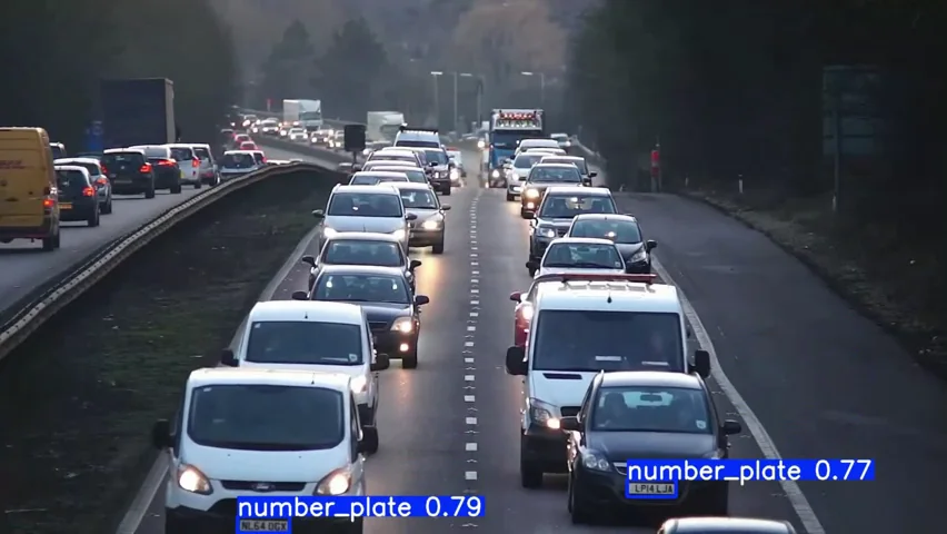
Output of my trained model on a test clip: the plates of the two nearest vehicles are detected with 0.79 and 0.77 confidence.

The frame also shows something the validation numbers don't. The model reliably finds plates close to the camera, but plates further back are only a few pixels tall in this 852×480 clip, and it doesn't detect them. Validation images look like the training set; real footage is a different test. For a real ANPR camera, higher resolution or a camera closer to the lane matters as much as the model. You can watch the full demo video on LinkedIn.

To use the detections in your own code, read the boxes from the results:

for box in results[0].boxes:
    x1, y1, x2, y2 = box.xyxy[0].tolist()
    print(f"class={int(box.cls)} conf={float(box.conf):.2f} box=({x1:.0f}, {y1:.0f}, {x2:.0f}, {y2:.0f})")

Step 7: Export for deployment

For production, export the model to a format your target runtime understands:

model.export(format="onnx")

ONNX runs almost anywhere, including CPU servers. Other options include engine (TensorRT, for NVIDIA GPUs and Jetson boards), tflite (mobile) and openvino (Intel CPUs).

What went wrong in my training

The numbers in this post come from my third training run. Ultralytics names each new run folder train, train2, train3, so the history is right there in runs/detect/.

• Colab disconnected mid-training. Free Colab sessions don't last forever, and a 50-epoch run takes hours. Resuming from last.pt (see Step 4) saved me from restarting from scratch.
• The first results weren't good enough. My first run didn't reach the accuracy I wanted, so I changed the training settings and trained again. The final run used the settings shown in Step 4.

What I'd tell myself before starting: save to Drive from the beginning, and when a run disappoints, change one setting at a time and compare the results.csv files. Otherwise you can't tell which change actually helped.

Common problems and fixes

• "Dataset not found": the paths in data.yaml are wrong. Use an absolute path: like /content/dataset and check the folder names match (valid vs val is a classic).
• CUDA out of memory: lower batch (16 → 8) or use batch=-1.
• Zero or very low mAP: usually a labelling problem. Check that label files have the same names as the images, that coordinates are normalised to 0–1, and that class indices match data.yaml.
• Good validation scores, poor results on real footage: the training images don't look like the real camera. Add images from the actual setting: same angle, lighting and resolution.
• Training is slow: confirm the GPU is active (Step 1), and keep the dataset on Colab's local disk rather than reading it from Drive.

Where to go next

• Compare model sizes: train yolov8s.pt with the same data and see whether the accuracy gain is worth the extra size and latency.
• The same workflow works for newer Ultralytics models such as YOLO11: change the weights file (for example yolo11n.pt) and keep everything else.
• Check the licence before commercial use: Ultralytics models are released under AGPL-3.0, with a separate enterprise licence for closed-source products.

The trained weights (best.pt) and detection script for this guide are on GitHub, and the full design decisions, training curve and next steps are in the car number plate detection case study.